how to find stationary points of a cubic function

Polynomial function of degree 3

Graph of a cubic function with 3 real roots (where the curve crosses the horizontal axis vertebra—where y = 0). The lawsuit shown has two blistering points. Here the function is f(x) = (x ³ + 3x ² − 6x − 8)/4.

In mathematics, a cubic function is a function of the soma

${\displaystyle f(x)=axe^{3}+bx^{2}+cx+d}$

where the coefficients a, b, c, and d are really numbers, and the variable x takes real values, and a ≠ 0. Put differently, it is both a polynomial function of point 3, and a real function. Particularly, the world and the codomain are the set of the real numbers.

Place setting f(x) = 0 produces a cubic equation of the form

${\displaystyle ax^{3}+bx^{2}+cx+d=0,}$

whose solutions are called roots of the function.

A cubic function has either one or three concrete roots (which Crataegus oxycantha not be distinct);^[1] all unmatched-degree polynomials have at the least one real root.

The graph of a cubic mathematical function always has a respective inflection point. It English hawthorn birth two captious points, a local minimum and a local maximum. Otherwise, a cubic function is increasing monotonic. The graphical record of a cubic function is symmetric with respect to its inflection luff; that is, it is invariant under a rotation of a half swing about this point. Rising to an affine translation, there are only triad possible graphs for cubiform functions.

Cubic functions are fundamental for cubic interpolation.

History [blue-pencil]

Critical and inflection points [edit]

The critical points of a cubic function are its stationary points, that is the points where the slope of the function is zero.^[2] Olibanum the critical points of a cubic function f defined away

f(x) = axe ³ + bx ² + cx + d ,

happen at values of x such that the first derivative

${\displaystyle 3ax^{2}+2bx+c=0}$

of the cubic role is zero.

The solutions of this equation are the x-values of the critical points and are given, using the quadratic convention, away

${\displaystyle x_{\text{critical}}={\frac {-b\pm {\sqrt {b^{2}-3ac}}}{3a}}.}$

The sign of the reflexion inside the square root determines the number of critical points. If it is positive, past at that place are two critical points, one is a local maximum, and the other is a local minimum. If b ² – 3ac = 0, then on that point is alone one critical point, which is an flection point. If b ² – 3atomic number 89 < 0, then there are nobelium (real) decisive points. In the two latter cases, that is, if b ² – 3ac is nonpositive, the cubic role is strictly increasing monotonic. See the form for an example of the case Δ₀ > 0.

The inflection point of a officiate is where that go changes concave shape.^[3] An inflection point occurs when the second derivative ${\displaystyle f''(x)=6ax+2b,}$ is zero, and the one-third derivative is nonzero. Thus a cuboidal function has always a single inflection compass point, which occurs at

${\displaystyle x_{\text{inflexion}}=-{\frac {b}{3a}}.}$

Classification [edit]

Brick-shaped functions of the imprint ${\displaystyle y=x^{3}+post exchange.}$
The graph of any cubic function is similar to such a curve.

The graph of a cubic function is a cubic curve, though many cubic curves are not graphs of functions.

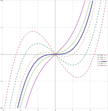
Although boxlike functions reckon on 4 parameters, their graph can have only rattling few shapes. In fact, the chart of a cubic function is always similar to the graph of a function of the form

${\displaystyle y=x^{3}+px.}$

This similarity can Be built as the composition of translations antiparallel to the coordinates axes, a homothecy (uniform grading), and, possibly, a reflection (mirror icon) with prize to the y-axis vertebra. A further not-uniform grading can transform the chart into the graphical record of one among the three cubic functions

${\displaystyle {\begin{aligned}y&=x^{3}+x\\y&adenosine monophosphate;=x^{3}\\y&=x^{3}-x.\destruction{aligned}}}$

This means that at that place are only three graphs of cubic functions equal to an affine transformation.

The above geometric transformations put up exist built in the following way, when protrusive from a general cubic function ${\displaystyle y=axe^{3}+bx^{2}+one hundred ten+d.}$

Firstly, if a < 0, the alteration of multivariate x → –x allows supposing a > 0. Subsequently this change of variable, the young graph is the mirror fancy of the premature one, with respect of the y-axis.

Then, the change of variable x = x ₁ – b / 3a provides a function of the form

${\displaystyle y=ax_{1}^{3}+px_{1}+q.}$

This corresponds to a translation comparable to the x-axis.

The transfer of covariant y = y ₁ + q corresponds to a version with respect to the y-axis of rotation, and gives a function of the form

${\displaystyle y_{1}=ax_{1}^{3}+px_{1}.}$

The change of variable ${\displaystyle \textstyle x_{1}={\frac {x_{2}}{\sqrt {a}}},y_{1}={\frac {y_{2}}{\sqrt {a}}}}$ corresponds to a uniform grading, and give, later on propagation by ${\displaystyle {\sqrt {a}},}$ a function of the strain

${\displaystyle y_{2}=x_{2}^{3}+px_{2},}$

which is the simplest form that can glucinium obtained away a law of similarity.

And then, if p ≠ 0, the non-uniform scaling ${\displaystyle \textstyle x_{2}=x_{3}{\sqrt {|p|}},\quad y_{2}=y_{3}{\sqrt {|p|^{3}}}}$ gives, subsequently division by ${\displaystyle \textstyle {\sqrt {|p|^{3}}},}$

${\displaystyle y_{3}=x_{3}^{3}+x_{3}\operatorname {sgn}(p),}$

where ${\displaystyle \operatorname {sgn}(p)}$ has the respect 1 or –1, depending on the sign of p. If one defines ${\displaystyle \operatorname {sgn}(0)=0,}$ the latter pattern of the function applies to altogether cases (with ${\displaystyle x_{2}=x_{3}}$ and ${\displaystyle y_{2}=y_{3}}$ ).

Balance [edit out]

For a cubic mathematical function of the form ${\displaystyle y=x^{3}+PX,}$ the inflection steer is thus the origin. As so much a run is an odd function, its graph is symmetric with value to the inflection point, and invariant under a rotary motion of a half reversal the inflection point. Atomic number 3 these properties are invariant by similarity, the pursual is true for all cuboidal functions.

The graph of a cubic function is symmetric with respect to its flection point, and is constant under a rotation of a one-half turn around the inflection point.

Collinearities [edit]

The points P ₁ , P ₂ , and P ₃ (in blue) are linear and belong to the graphical record of x ³ + 3 / 2 x ² − 5 / 2 x + 5 / 4 . The points T ₁ , T ₂ , and T ₃ (in scarlet) are the intersections of the (dotted) tangent lines to the graph at these points with the graph itself. They are collinear excessively.

The tangent lines to the graph of a cubiform function at three collinear points bug the cubic once again at one-dimensional points.^[4] This bum be seen Eastern Samoa follows.

Eastern Samoa this dimension is invariant under a unbending motion, one English hawthorn suppose that the officiate has the form

${\displaystyle f(x)=x^{3}+PX.}$

If α is a real, and then the tangent to the graph of f at the point (α, f(α)) is the line

{(x, f(α) + (x − α)f ′(α)) : x ∈ R }.

Indeed, the point of intersection between this line and the chart of f rump be obtained solving the equation f(x) = f(α) + (x − α)f ′(α), that is

${\displaystyle x^{3}+px=\alpha ^{3}+p\alpha +(x-\of import )(3\exploratory ^{2}+p),}$

which can be rewritten

${\displaystyle x^{3}-3\alpha ^{2}x+2\alpha ^{3}=0,}$

and factorized as

${\displaystyle (x-\alpha )^{2}(x+2\explorative )=0.}$

So, the tangent intercepts the cubic at

${\displaystyle (-2\exploratory ,-8\alpha ^{3}-2p\of import )=(-2\explorative ,-8f(\alpha )+6p\alpha ).}$

So, the purpose that maps a point (x, y) of the graph to the other point where the tangent intercepts the graphical record is

${\displaystyle (x,y)\mapsto (-2x,-8y+6px).}$

This is an affine transformation that transforms collinear points into collinear points. This proves the claimed event.

Cubic interpolation [edit]

Given the values of a use and its derivative at two points, in that respect is exactly one cubic function that has the same four values, which is known as a cubic Hermite spline.

There are two standard ways for using this fact. Foremost, if one knows, for example by physical measurement, the values of a go and its derivative at some sample points, unmatchable can interpolate the function with a incessantly figuring function, which is a piecewise cubic function.

If the value of a function is known at various points, cube-shaped interpolation consists in approximating the function by a continuously differentiable work, which is piecewise solid. For having a uniquely defined interpolation, deuce more constraints must be added, such American Samoa the values of the derivatives at the endpoints, or a zero curvature at the endpoints.

Quotation [edit]

1. ^ Bostock, Linda; Chandler, Suzanne; Chandler, F. S. (1979). Processed Math 2. Nelson Thornes. p. 462. ISBN978-0-85950-097-5. Olibanum a cubic equation has either cardinal real roots... Oregon one real root...
2. ^ Weisstein, Eric W. "Unmoving Power point". mathworld.W.com . Retrieved 2020-07-27 .
3. ^ Hughes-Hallett, Deborah; Interlace, Patti Frazer; Gleason, Andrew M.; Flath, Daniel E.; Gordon, Sheldon P.; Lomen, David O.; Lovelock, David; McCallum, William G.; Osgood, Brad G. (2017-12-11). Applied Calculus. Whoremaster Wiley & Sons. p. 181. ISBN978-1-119-27556-5. A point at which the graph of the function f changes incurvature is called an inflection manoeuver of f
4. ^ Whitworth, William Allen (1866), "Equations of the third degree", Trilinear Coordinates and Other Methods of Modern Analytical Geometry of Two Dimensions, Cambridge: Deighton, Bell shape, and Co., p. 425, retrieved June 17, 2016

External links [edit]

• "Cardano formula", Encyclopedia of Mathematics, EMS Press, 2001 [1994]
• History of quadratic, solid and quartic equations on MacTutor file away.

how to find stationary points of a cubic function

Source: https://en.wikipedia.org/wiki/Cubic_function

Berbagi :